Our Blog

Exploring Geodatabase Files

By Constante “Tino” Gonzalez
August 14, 2024

One of our clients recently provided us with a dataset of real estate properties that they manage, and asked us to generate content based off of the points and polygons in the dataset.

We will walk through the process of extracting polygons, placemarks, and other info from a geodatabase file and converting them into separate KML files using the ogr2ogr command-line tool, adding some logic to the data selection to limit the subset of features. We will also explore the GDB file using the GDAL Python library to export the data as JSON for use in other scripts.

Prerequisites

• Basic understanding of geospatial data
• Installed versions of the GDAL/OGR library
• A geodatabase file (.gdb, .gdb.zip, or .shp)

A first look into the contents of the GDB file

ogrinfo example.gdb.zip

This command will list all layers that are available in the dataset. Add a specific layer as a parameter to the same command, and it will output all the fields, their types, and values for every feature in the layer.

ogrinfo example.gdb.zip a_layer_name

The parameter -so can be used to omit the values from the output and get only the layer field names and types:

#$> ogrinfo example.gdb.zip Land_Points -so
INFO: Open of `example.gdb.zip'
      using driver `OpenFileGDB' successful.

Layer name: Land_Points
Geometry: Point
Feature Count: 219
Extent: (-122.699891, -23.590280) - (139.763352, 59.622821)
Layer SRS WKT:
GEOGCRS["WGS 84",
    DATUM["World Geodetic System 1984",
        ELLIPSOID["WGS 84",6378137,298.257223563,
            LENGTHUNIT["metre",1]]],
    PRIMEM["Greenwich",0,
        ANGLEUNIT["degree",0.0174532925199433]],
    CS[ellipsoidal,2],
        AXIS["geodetic latitude (Lat)",north,
            ORDER[2],
        ANGLEUNIT["degree",0.0174532925199433]],
    USAGE[
        SCOPE["unknown"],
        AREA["World"],
        BBOX[-90,-180,90,180]],
    ID["EPSG",4326]]
Data axis to CRS axis mapping: 2,1
FID Column = OBJECTID
Geometry Column = Shape
asset_type: Integer (0.0)
asset_id: String (15.0)
property_code: String (255.0)
full_address_text: String (255.0)
land_name: String (255.0)
land_address1: String (255.0)
land_city: String (255.0)
land_sate_code: String (50.0)
land_postal_code: String (10.0)
land_country_code: String (50.0)
division_name: String (255.0)
region_name: String (255.0)
market_name: String (255.0)
submarket_name: String (255.0)
supplemental_portfolio_name: String (255.0)
ownership_name: String (255.0)
land_held_for_sale_acre: Real (0.0)
land_held_for_sale_hect: Real (0.0)
land_held_for_development_acre: Real (0.0)
land_held_for_development_hect: Real (0.0)
total_land_acre: Real (0.0)
total_land_hectare: Real (0.0)
buildable_area_sf: Real (0.0)
buildable_area_sm: Real (0.0)
buildable_area_tsubo: Real (0.0)
land_latitude: Real (0.0)
land_longitude: Real (0.0)
geocoded: Integer (0.0) DEFAULT 0
globalid: String (0.0) NOT NULL
created_user: String (255.0)
created_date: DateTime (0.0)
last_edited_user:  String (255.0)
last_edited_date: DateTime (0.0)

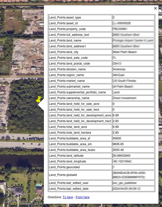
This command shows you information for a single layer, which can be helpful if you are only looking for certain values. However, the geographic data is not much to look at in the terminal. To visualize it, we can convert the data to KML, which applications like Google Earth or Cesium can render while keeping the information as text that can be read:

ogr2ogr -f "KML" example_output.kml example.gdb.zip layer_name

• -f "KML" specifies the output format
• example_output.kml is the name of the output KML file
• example.gdb.zip is the path to the geodatabase file
• layer_name is the geodatabase layer to export

This command will export into a KML file:

• All the geometries in the layer, be it placemarks or polygons in our case
• All the other fields of information as extended data, which will show up for each feature as a balloon table when visualized in Google Earth

The ogr2ogr -sql option

The default balloon popup was not the outcome we wanted for this KML file. We first used sed to remove all the extended data from the KML files, but after looking into it a bit further, we found an ogr2ogr option, -sql, that made the data filtering easier. This option lets us add a query to the command just like getting the data from a SQL database.

1. Extract property names

To create a KML file with just the names of the properties, look up the layers and fields in them using ogrinfo and find the points layer that has the names—in this case, Layer_Points. Then, add the desired SQL query to the command.

ogr2ogr -f "KML" output_names.kml example.gdb.zip -sql "SELECT name FROM Layer_Points"

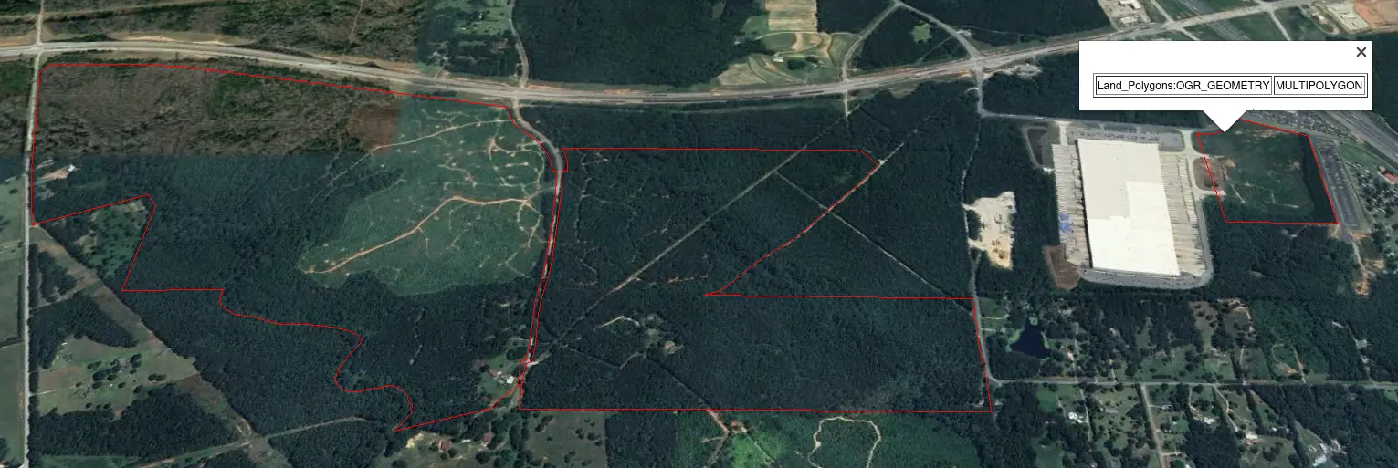
2. Extract polygons only

The polygon geometries are stored in Layer_Polygons. They can be selected using the special OGR field OGR_GEOMETRY that refers to the geometry of the selected layer:

ogr2ogr -f "KML" output_polygons.kml example.gdb.zip -sql "SELECT OGR_GEOMETRY FROM Layer_Polygons"

3. Create KML with pins and names

To create a KML file with property names as placemarks with pins, we just select the name. The point placemark seems to be included with all data:

ogr2ogr -f "KML" output_pins.kml input.gdb layer_name -sql "SELECT name FROM layer_name"

4. Create KML with pins only, no names

To get the points with nothing else, we use the SQLite MakePoint function, which selects a list of points from the KML.

ogr2ogr -f "KML" output_pins.kml input.gdb layer_name -dialect SQLite -sql "SELECT MakePoint(land_longitude, land_latitude) AS geom FROM Land_Points"

5. Extract limited properties

For extracting a limited number of properties, we can add the WHERE clause to the SQL command:

ogr2ogr -f "KML" output_pins.kml input.gdb layer_name -sql "SELECT name FROM layer_name"

We can also use the ogr2ogr -where flag to use that part of the query only:

ogr2ogr -f "KML" limited_output_polygons.kml input.gdb layer_name -where "ID IN (1, 2, 3)"

6. Run it all in a Python script

There is a Python GDAL library, which I will cover the basics of later, but first, here is a simplified example using Python subprocess to run the ogr2ogr commands we tested in the terminal.

import subprocess

gdb_file = "example.gdb.zip"
column_name = "p_code"
elem_str = "'a1', 'a2', 'b1', 'b3'"

sql_land_labels = f"SELECT land_name FROM Land_Points WHERE {column_name} IN ({elem_str})"
subprocess.run(['ogr2ogr', '-f', 'KML', 'land_labels.kml', gdb_file, '-sql', sql_land_labels])

sql_land_points = f"SELECT MakePoint(land_longitude, land_latitude) AS geom FROM Land_Points WHERE {column_name} IN ({elem_str})"
subprocess.run(['ogr2ogr', '-f', 'KML', 'land_points.kml', gdb_file, '-dialect', 'SQLite', '-sql', sql_land_points])

sql_land_polygons = f"SELECT OGR_GEOMETRY FROM Land_Polygons WHERE {column_name} IN ({elem_str})"
subprocess.run(['ogr2ogr', '-f', 'KML', 'land_pols.kml', gdb_file, '-sql', sql_land_polygons])

This script will create the three different KML files that we usually need for our presentations. We used variables for the gdb_file, column_name, and elem_str command line parameters to make the script easy to use for selecting other data. We also use them in other scripts to join, apply custom styling, and add regions to the KMLs, which will be covered in another blog post.

7. Extract all data as JSON from one layer using the Python GDAL library

I probably should have started here, but I only used the Python library later on in the process to join the gdp.zip file data with data from other sources (spreadsheets, emails, etc.).

First, install the GDAL library:

pip install gdal

Then you can use the following Python script, changing as necessary the gdb_file, layer_name, and the unique field chosen to structure the data. The code is explained in the comments.

#!/bin/python

import json
from osgeo import ogr

# Open the Geodatabase file
driver = ogr.GetDriverByName('OpenFileGDB')
gdb_file = 'example.gdb.zip'
data_source = driver.Open(gdb_file, 0)

# Get the layer
layer_name = 'Building_Points'
layer = data_source.GetLayerByName(layer_name)
if layer:
    # Get the layer definition
    layer_defn = layer.GetLayerDefn()

    # Get the number of fields in the layer
    num_fields = layer_defn.GetFieldCount()

    # Initialize an empty list to store field names
    field_names = []

    # Iterate over each field and add its name to the list
    for i in range(num_fields):
        field_defn = layer_defn.GetFieldDefn(i)
        field_name = field_defn.GetName()
        field_names.append(field_name)

    print("Field names:", field_names)
else:
    print(f"Layer '{layer_name}' not found.")

all_info = {}

# Iterate over all features and organize all field names under a unique one for the dictionary structure
for feature in layer:
    if feature is not None:
        globalid = feature.GetField('globalid')
        all_info[globalid] = {}
        for fn in field_names:
            all_info[globalid][fn] = feature.GetField(fn)

# Close the data source
data_source = None

# Save information to a JSON file
output_file = 'info.json'
with open(output_file, 'w') as json_file:
    json.dump(all_info, json_file, indent=4)
print(f"Information saved to {output_file}")

The script will create a JSON file with all the information on the layer.

Conclusion

Following these steps, we can efficiently manage and visualize geospatial data using ogr2ogr, SQL, and KML, and in some cases, JSON. These methods allow for a high degree of customization and can be tailored to specific project requirements.

Additional Resources

• GDAL/OGR Documentation
• GDAL Python Bindings
• KML Documentation
• SQLite Documentation

gis python google-earth open-source visionport